Transmission ratio through single barrier (Python3)
Transmission
ratio (t) of a particle through single barrier is calculated and shown by
Python3. This is preparation for another case of double barriers and a quantum well shown in the next page.
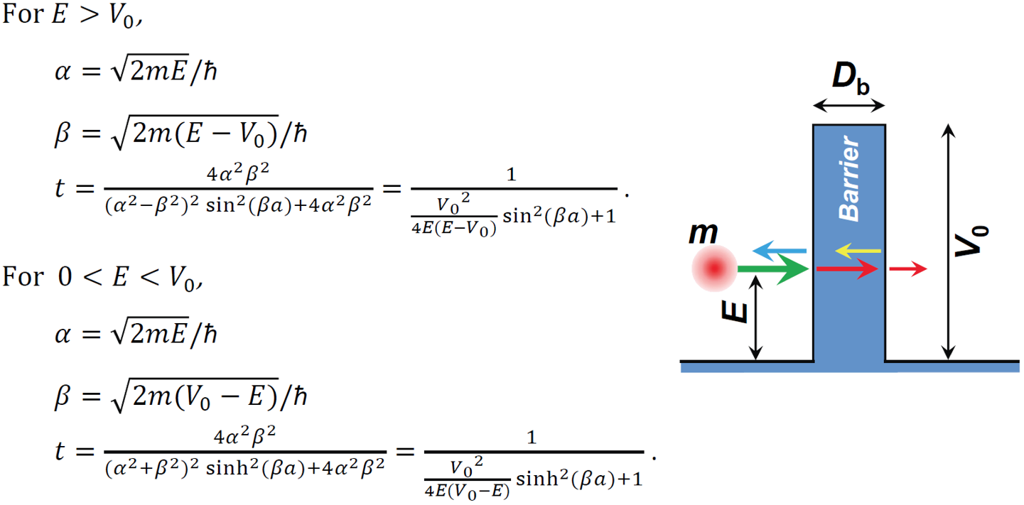
Following equations used here are a set of solution obtained by one-dimensional Schrödinger
equation with typical initial condition. Height (V0) and thickness (a = Db) of the
barrier are 0.5 eV and 2.8 nm, respectively. Effective mass (m) of a
particle is 0.35 m0 (m0:
electron mass in vacuum).
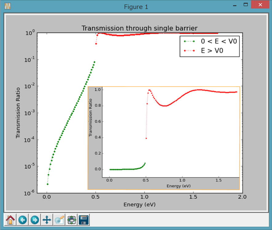
Quantum tunneling can be observed at lower energy below the barrier height (the green plots). Additionally, even at higher energy beyond the barrier height (the red plots), lowering of transmission ratio due to scattering is clearly shown.
| # Tunneling_single_barrier_01.py # on Python 3.4.1, Nov. 29, 2014 # by Masao Sakuraba import math import numpy import scipy import pylab def main(): meff = 0.35 # effective mass ratio of a particle V0 = 0.5 # barrier height (eV) Db = 2.5e-9 # barrier thickness (m) q = 1.602e-19 # elementary charge (C) hbar = 1.0546e-34 # reduced Planck constant (J s) hbar2 = hbar ** 2 m = meff * 9.1095e-31 # absolute mass of a particle (kg) # parameters for lower energy (0 < E < V0) M = 50 # number of energy step Alpha_d = [] Alpha_d2 = [] Beta_d = [] Beta_d2 = [] Sinh = [] Sinh2 = [] t_d = [] # parameters for higher energy (E > V0) N = 100 # number of energy step Alpha_u = [] Alpha_u2 = [] Beta_u = [] Beta_u2 = [] Sin = [] Sin2 = [] t_u = [] E_d = numpy.linspace(V0 / M, V0 - V0 / M, M - 1) for i in range(M - 1): Alpha_d2.append(2 * m / hbar2 * E_d[i] * q) Alpha_d.append(math.sqrt(Alpha_d2[i])) Beta_d2.append(2 * m / hbar2 * (V0 - E_d[i]) * q) Beta_d.append(math.sqrt(Beta_d2[i])) Sinh.append(numpy.sinh((Beta_d[i]) * Db)) Sinh2.append(Sinh[i] ** 2) t_d.append( 4 * Alpha_d2[i] * Beta_d2[i] / ((Alpha_d2[i] + Beta_d2[i]) ** 2 * Sinh2[i] + 4 * Alpha_d2[i] * Beta_d2[i]) ) E_u = numpy.linspace(V0 + V0 / N, V0 * 3.5 - V0 / N, N - 1) for j in range(N - 1): Alpha_u2.append(2 * m / hbar2 * E_u[j] * q) Alpha_u.append(math.sqrt(Alpha_u2[j])) Beta_u2.append(2 * m / hbar2 * (E_u[j] - V0) * q) Beta_u.append(math.sqrt(Beta_u2[j])) Sin.append(math.sin(Alpha_u[j] * Db)) Sin2.append(Sin[j] ** 2) t_u.append( 4 * Alpha_u2[j] * Beta_u2[j] / ((Alpha_u2[j] - Beta_u2[j]) ** 2 * Sin2[j] + 4 * Alpha_u2[j] * Beta_u2[j]) ) # 'option' : color (r,g,b,c,m,y,k,w) & line style (-,--,:,-.,.,o,^) pylab.plot(E_d, t_d, 'g:.', label='0 < E < V0') pylab.plot(E_u, t_u, 'r:.', label='E > V0') pylab.legend(loc='upper right') pylab.title('Transmission through single barrier') pylab.xlabel('Energy (eV)') pylab.ylabel('Transmission Ratio') pylab.xlim(-0.1, V0 * 4) pylab.yscale('log') # Delete this line, if linear y. # pylab.ylim(-0.1, 1.4) pylab.show() if __name__ == '__main__': main() |
This home page is produced by KompoZer (free and open software).